转录相互作用

• 1 网络模体（结构单元模式）
• 2 最简单的网络模体：负自身调节模块
• 3 模体的作用及稳定

第一部分

随机化网络和调控网络比较，找出统计学显著性有意义的模式，即为网络模体。

生物体碱基序列的突变会为网络增添或者减少边的个数。

经典的随机网络模型为 Erdos-Renyi（ER）模型，与调控网络的边E和节点数N相同，每一个可能的边的位置被占用的概率为$p=\frac{E}{N(N-1)+N}$,即$\frac{E}{N^2}$。

%matplotlib inline
对于上述命令行的疑问解答
ipython中有一类型的magic function，属于内嵌函数,用于绘图，pycharm不支持，但是在ipython（jupyter notebook）中使用，可以省略plt.show()步骤，在当前行一下使用。

P3 监督学习

correct answers

in every example in our data set, we are told what is the “correct answer” that we would have quite liked the algorithms have predicted on that example, such as the prices of the house or whether the tumor is malignant or benign.

Regression：预测连续性变量的输出，predict continuous valued output(price)
eg: sell house，breast cancer

Classification: discrete valued output(0 or 1) eg：breast cancer: use tumor size and age to predict malignant or benign

inifinite number of features
SVM: allow computer to deal with an infinite number of features to aviode memory error.

无监督学习

不知道分类或者聚类的结果
clustering
cocktail party problem

使用octave的优势。

模型描述

m: number of training examples

$x^s$: “input” variable/feature

$y^s$: “output” variable/“target” variable

cost function（代价函数）

Hypothesis: $h^{\theta}(x)=\theta_0+\theta_1x$

Cost function: $J({\theta}0,{\theta}_1)={\frac{1}{2m}}{\times}{\sum(h{\theta_0}(X^{(i)})-y^{(i)})^2}$

contour plot

找到$\theta0$,$\theta1$，使得J最小。

梯度下降

目的：找到$\theta_0$,$\theta_1$，使得J最小。

从不同的角度出发，会获得不同的局部最优解。

梯度下降时要求同时更新$\theta_0$,$\theta_1$，其中$\alpha$后面的一项是J($\theta_0$,$\theta_1$),在$\theta_0$,$\theta_1$切线的斜率。learninng rate $\alpha$:越大表示梯度下降越快。

当接近局部最小值的时候，梯度下降会自动减小步幅，所以不用一直减小$\alpha$。

梯度下降算法的推导

将线性回归的J 函数带入梯度下降的公式，可以推导出$\theta_0$,$\theta_1$，这时候平方和求导抵消，因此没有平方。

凸函数只有全局最优解，没有局部最优解

Batch gradient descent algorithm

batch: each step of gradient descent uses all the training examples

3-1 Linear Algebra review: matrices and vectors

matrix: rectangular array of numbers

dimension of matrix: number of rows X number of columns

vector: An nX1 matrix

3-2 Linear Algebra review: Addition and scalar multiplication

矩阵加减以及和一个常量乘除，和数字的运算一致，逐个元素相加相减。

3-3 Linear Algebra review: matrix-vector multiplication

解方程的矩阵代入

3-3 Linear Algebra review: matrix-matrix multiplication

解方程的矩阵代入

3-4 Linear Algebra review: matrix multiplication properties

矩阵相乘没有交换率(communitive)

矩阵相乘符合结合律（asscociation)

identify matrix: $A I =I A =A$,I即为 单位矩阵，维数通常隐藏的。

倒数矩阵

3-4 Linear Algebra review: Inverse and transpose

4-1 Linear Regression with multiple variables: Multiple variables

多元回归的函数

4-2 Linear Regression with multiple variables: Gradient descent for multiple variables

4-2 Linear Regression with multiple variables: Gradient descent in practice I: Feature Scaling

Feature scaling
idea: make sure features are on a similar scale
如果两个变量的范围量级差异很大，会造成梯度函数的等高图变成椭圆形，学习时，振荡范围很小，导致学习时间巨长。一般性控制全部变量的取值范围在-3~3区间即可

mean normalization：X=(x-u)/(max-min)
特征缩放不用非常精确，因为目的只是让梯度下降更快一点。

4-3 Linear Regression with multiple variables: Gradient descent in practice II: Leanring rate

对于线性回归，当学习率足够小，每一次迭代后J($\theta$)会一直递减，、。

学习率过大：J($\theta$)上升或者波动，不收敛。
学习率过小：收敛速度很慢。

在选择学习率的时候，需要打印J($\theta$)函数。tricky：可以以3倍的速度进行选择，尝试最大值和最小值后，在最大值附近选取一个合适的学习率。（…0.001，0.003，0.01，0.03，0.1，0.3，1…）

4-4 Linear regression with multiple variables:Features and polynomial regression

可以选择多种函数来fit the curve

4-5 Linear regression with multiple variables: Normal equation(正规方程，区别于迭代方法的直接解法)

J($\theta$)在$\theta$的导数=0
$\theta$=pinv(X’X)X’y X’倒置。pinv求倒数
对于正规方程，不用feature scaling.

4-5 Linear regression with multiple variables: Normal equation and non-invertibility

$\theta$=pinv(X’X)X’y 如果X’X不能求倒数，即为singular/degenerate 矩阵。
Octave：pinv()和inv()都是求倒数，但是pinv能够求解奇异矩阵的倒数，是pseudo inv.

X’X不能求倒数的可能原因：

Logistic regression： Classfication

回归不适合分类。
Classfication: y=0 or y=1
h(x) can be >1 or <1
logistic regression: 0<=h(x)<=1 用于classification。

Logistic regression: Hypothesis representation

want 0<=h(x)<=1

sigmoid function = logistic function

hθ(x)=g(θTx)
z=θTx
g(z)=1/(1+e−z)

hθ(x)=P(y=1|x;θ)=1−P(y=0|x;θ)P(y=0|x;θ)+P(y=1|x;θ)=1

Logistic regression: Decision boundary

y=1, θTx>=0;
y=0, θTx<0

Non-linear decision boundaries

Logistic regression: simplified cost function and gradient descent

Logistic regression: Advanced optimization

The probekm of overfitting

Unfit, high bias: too sample or use too few features

Overfiting, high variance: a compllicated function that creates alot of unnecessary curves and angles unrelated to the data
多幂函数的产生，用力拟合，cost function 很小，但是不具备广泛的拟合。

adressing overfiting,feature 太多，并且训练集太少会导致overfiting

• 1. reduce number of features
• manually select which features to keep)
• model selection algorithm(later in course)
• 2. regularization
• keep all the features,but reduce magnitude/values of parameters theta
• works well when we have a lot of features,each of which contributes a bit to predicting y.

Regularization: cost function

为了避免过度拟合（往往由高阶幂造成），在cost function上加一个参数项$\lambda$ $\theta$，如果参数项越大，训练的目的是使cost function 小，所以会设置$\lambda$非常大，$\theta$约等于0，就能减少cost function。
$\theta0$，$\theta1$，$\theta2$…$\theta$n越小，拟合的曲线越光滑。

正则化的项，是为了平衡拟合训练的目的以及近可能保持低的$\theta$值

Regularization Linear Regression

Week 4 model representation I

$a^{(j)i}$=”activation” of unit i in layer

$Θ^{(j)}$=matrix of weights controlling function mapping from layer j to layer j+1

dim($Θ^{(j)}$)=$S_{j+1}$ *$S_{j}+1$

Week 5 Neural Network Learning: Unrolling Parameters

为了使用优化函数，要求变量是向量，而神经网络中$\theta$是矩阵而非向量，因此可以卷开为thetaVec，梯度也需要卷开。

Week 5 Neural Network Learning: Gradient checking

目的：减少代码错误

Week 5 Random Initialization

初始化theta参数，需要随机取值，否则如果theta1=theta 2 ,会造成symmetry breaking。

问题

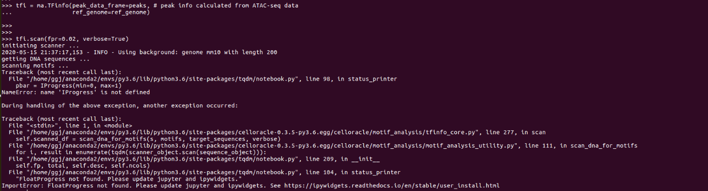
使用CellOracle的时候，报错“InProgress is not defined”

解决方法1

网上给出的解决方式是在base环境（安装jupyter）中安装widgetsnbextension，在使用环境安装ipywidgets，具体可以见网址 https://ipywidgets.readthedocs.io/en/stable/user_install.html ，但是这个方法对我不适应。

解决方法2

实测有效

使用jupyter notebook 来跑程序，但是出现kernel keep die的情况，那么需要卸载ipykernel和ipython，然后重新，并且安装nb_conda(为了是jupter识别该conda环境),参考网址：https://github.com/tqdm/tqdm/issues/872

1
2
3
4
5

conda remove ipykernel
conda remove ipython
conda install ipykernel
conda install ipython
conda install nb_conda

分析流程

1. ATAC-seq data preprocessing

目的： identify accessible promoter/enhancer DNA regions

scATAC-seq: proximal and distal promoter/enhancer genome sequences(co-accessible socres and TSS infomation)

bulk ATCC seq: proximal promoter/enhancer genome sequences

输入：ATAC的结果，以bed file的形式

输出：peaks,gene_short_name,co-access scores(bulk无)

2. Transcription factor binding motif scan

目的： 扫描基因的调控序列，获取TF list
输出：矩阵，行peaks name and target gene name, 列TF names

3. scRNA-seq data preprocessing with scanpy or seurat

4. Network analysis

数学期望的定义：

离散型随机变量的数学期望是概率值*取值的绝对值的求和

连续性随机变量：先决条件：x的绝对值乘以密度函数的积分绝对收敛

不同分布的数学期望

泊松分布：X~P(\lambda)
二项分布:
指数分布
正态分布：u
柯西分布：数学期望不存在

随机变量函数的数学计算

实际背景问题：随机变量可测量，密度函数已知，另外一个随机变量有关，但是不可测量。

计算公式：f(x)乘以g(x)在x取值范围的积分即可

参考的网址

科学网 周涛 2012年关于复杂网络的入门书籍和review 介绍

http://blog.sciencenet.cn/blog-3075-549946.html

周涛 2017年关于复杂网络的review 推荐

https://blog.csdn.net/An_Wu/article/details/78653044?utm_medium=distribute.pc_relevant.none-task-blog-BlogCommendFromMachineLearnPai2-15.nonecase&depth_1-utm_source=distribute.pc_relevant.none-task-blog-BlogCommendFromMachineLearnPai2-15.nonecase

CSDN 博客 复杂网络入门笔记

https://blog.csdn.net/SHU15121856/article/details/70199009

网络参数的解读

• 1. Degree distributions：node连接的edges的数量。
• 2. Neighborhood connectivity: neighbors 的数量

• Stress centrality：构建最短路径经过的数量

• Betweenness centrality：

degree centrality is the most straightforward measure, reporting how many edges are connected to a node (in this case, how many genes a given TF connects to)

betweenness centrality and eigenvector centrality; genes with high betweenness are essential for the transfer of information within a network, whereas genes with high eigenvector centrality scores have the most substantial influence in terms of their connections to other well-connected genes

参考网址

搭建博客参考网址：https://www.cnblogs.com/selier/p/9568165.html 或者http://stevenshi.me/2017/05/07/hexo-blog
theme-next 主题修改：http://theme-next.iissnan.com/getting-started.html
图库搭建:https://www.cnblogs.com/ly-2019/p/11828790.html
博客升级参考；https://www.jianshu.com/p/9f0e90cc32c2

简单命令

1
2
3
4
5

hexo new "文章标题"
hexo g  ## 生成静态网页
hexo s  ## 本地浏览
hexo d  ## 部署到github
hexo clean ##清除缓存文件db.json和已生成的静态文件public

Welcome to Hexo! This is your very first post. Check documentation for more info. If you get any problems when using Hexo, you can find the answer in troubleshooting or you can ask me on GitHub.

Quick Start

Create a new post

1

$ hexo new "My New Post"

More info: Writing

Run server

1

$ hexo server

More info: Server

Generate static files

1

$ hexo generate

More info: Generating

Deploy to remote sites

1

$ hexo deploy

More info: Deployment